AI-Powered Pill Counting: Real-Time Vision for High-Speed Pharmaceutical Lines

A pharmaceutical manufacturer needed a direct, verifiable count of solid dose units discharging from a sloped chute into packaging containers, at roughly fifteen to twenty units per second across two product formats. Three constraints shaped everything: run completely offline, use only components licensed for commercial use, and deploy without modifying the mechanical line.

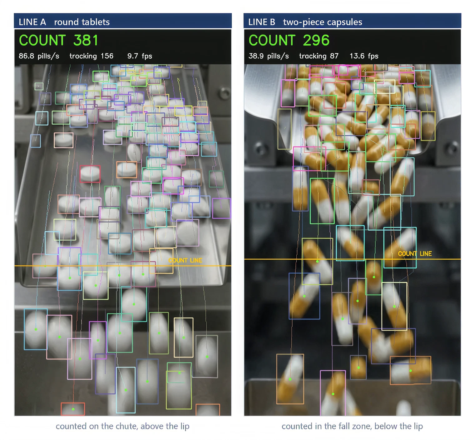
The solution pairs a compact, purpose-trained detection network with a motion-aware tracker and a line-crossing counter. Rather than detecting bounding boxes and resolving overlaps afterwards — which fails predictably when objects are dense, identical and touching — the model predicts a centre-point heatmap, separating adjacent units by construction. Every count is cross-checked by an independent estimator that never touches the tracker.

The result is a 0.32-million-parameter detector in a 1.3 MB deployment file that sustains real-time counting on an ordinary CPU and scales to several camera streams on one GPU workstation, with no cloud dependency and no copyleft obligation on the shipped product. Against hand-verified ground truth on held-out benchmark clips, the fully trained tablet detector recovered 99.1 per cent of units.

The Business Challenge

Solid dose packaging is one of the few places in manufacturing where the thing being controlled — the number of units in a container — is rarely measured directly.

Why Indirect Counting Becomes a Problem

Weight-based inference is blind to unit variation: Checkweighing resolves a miscount only when the mass difference exceeds natural tablet-to-tablet variation. For small units a single missing item sits inside the noise band.

Reconciliation happens after the fact: It catches an aggregate discrepancy, but by then the containers are downstream — the corrective action is investigation, not prevention.

Manual verification does not scale to line speed: At twenty units per second no operator can verify a count visually, so most containers are never independently checked.

Every discrepancy is a documentation event: The cost is not only the product; it is the deviation record, the investigation and the staff time to close it out.

What the Line Actually Needed

A continuous, per-unit count at the point of discharge, available in real time and reliable enough to serve as an in-process control — observing the process without touching it: no hardware in the product path, no change to line speed, no additional cleaning validation.

Two constraints then shaped everything technical. The plant network is isolated, so nothing may call a cloud service or require a licence check to start. And the shipped software had to be free of copyleft obligations — several of the highest-profile open detectors carry terms unworkable for a commercial product. That ruled out the obvious shortcut and made a purpose-built model the correct answer.

The Operational Workflow Before AI

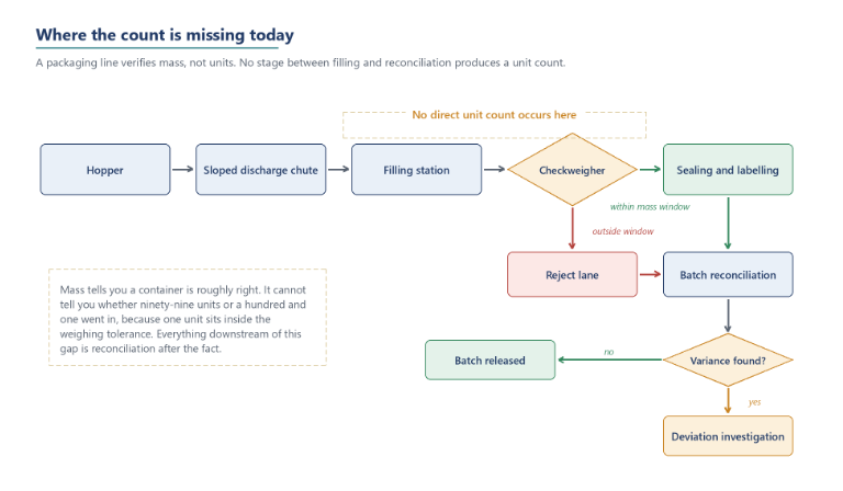
• Product is dispensed from the hopper onto a sloped chute, where units accelerate under gravity.
• A filling mechanism meters product into each container, targeting a nominal unit count.
• A checkweigher compares total mass against a window derived from average unit weight.
• Containers outside the mass window are rejected automatically.
• An operator performs periodic manual counts on sampled containers for the batch record.
• At batch close, units dispensed are reconciled against units packed, and variance is investigated.

Each step is sound in isolation. The gap is structural: nothing measures the count of every container, continuously, at the moment it is created.

This workflow is not broken; it is a mature, validated arrangement. The argument for direct counting is not that these controls fail, but that all three are indirect — none observes individual units.

Technical Challenges and Edge Cases

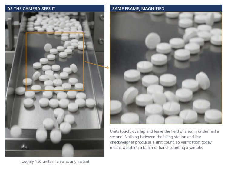
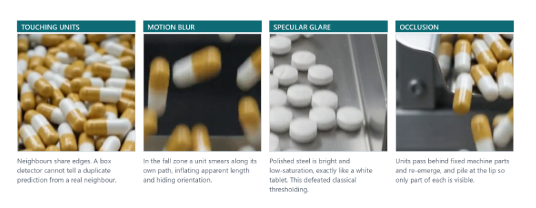
Objects are dense, identical and touching

A conventional box detector relies on non-maximum suppression to remove duplicates. That works when overlap means duplication. Here it does not: two heavily overlapping boxes are just as likely to be two touching tablets. Suppression then removes real objects, and relaxing it re-admits duplicates. No threshold resolves both, because the geometry is identical.

Motion blur and changing apparent scale

A unit can traverse a substantial fraction of its own diameter within one exposure. Because the camera views a sloped chute, units near the bottom of the frame are closer to the lens and faster than those at the top, so any method assuming a single object scale is wrong somewhere in the frame by construction.

Objects live for only a handful of frames

At the observed fall rate a unit is visible in the counting region for roughly five frames, so any tracker needing time to establish a motion model has none. This proved the most consequential constraint in the system.

Reflective steel, and two very different formats

The chute is polished metal and its highlights move with the product; a classical vision probe returned roughly fifty per cent more candidate regions than there were units. Accuracy testing later confirmed this quantitatively: every false positive the finished system produced came from reflections off conveyor side walls, on a single test clip. Round tablets and capsules also differ — capsules tumble and accelerate, roughly quadrupling their frame-to-frame displacement across the region.

No ground truth, and no budget for manual labels

A single ten-second clip at production density contains tens of thousands of instances. Hand-annotation was not viable, and partial annotation is actively harmful: an unlabelled object teaches the model that a real object is background.

The AI Solution

A single fixed camera feeds four cooperating stages, each addressing a failure mode above.

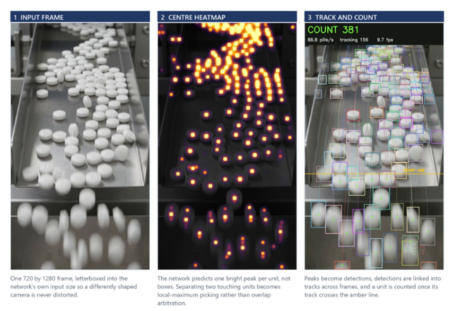
• A centre-point detector: The network predicts a heatmap in which each object contributes one peak at its centre, plus small maps giving its size and a sub-pixel correction. Two touching units produce two distinct peaks even when their outlines merge.

• A self-calibrating duplicate filter: Residual duplicate peaks are removed using a suppression radius derived from the model’s own predicted object size, so the filter adapts to the product rather than to a hard-coded distance.

• A motion-aware tracker: Detections are linked into persistent tracks, with gates scaled to predicted object size and new tracks initialised at the prevailing local velocity rather than from rest.

• A line-crossing counter: A track increments the count once, when its centre crosses a virtual line while supported by a live detection — preventing a coasting track from registering a phantom crossing.

• Two alternatives were rejected on evidence: classical image processing over-detected badly, and general-purpose pretrained detectors were usable offline but undeployable under copyleft licences. Two models are deployed, one per format, because the formats run on separate lines and two small models cost almost nothing to run.

The AI Development Pipeline

Data Collection

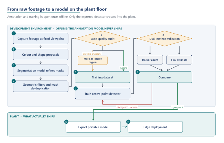
Footage was captured from a fixed viewpoint, cropped above the container so the scene contains only product in flight. Frame rate determines viability: tracking associates detections across consecutive frames, and at the observed speeds sixty frames per second yields roughly five observations per unit — the practical floor.

Automated Annotation

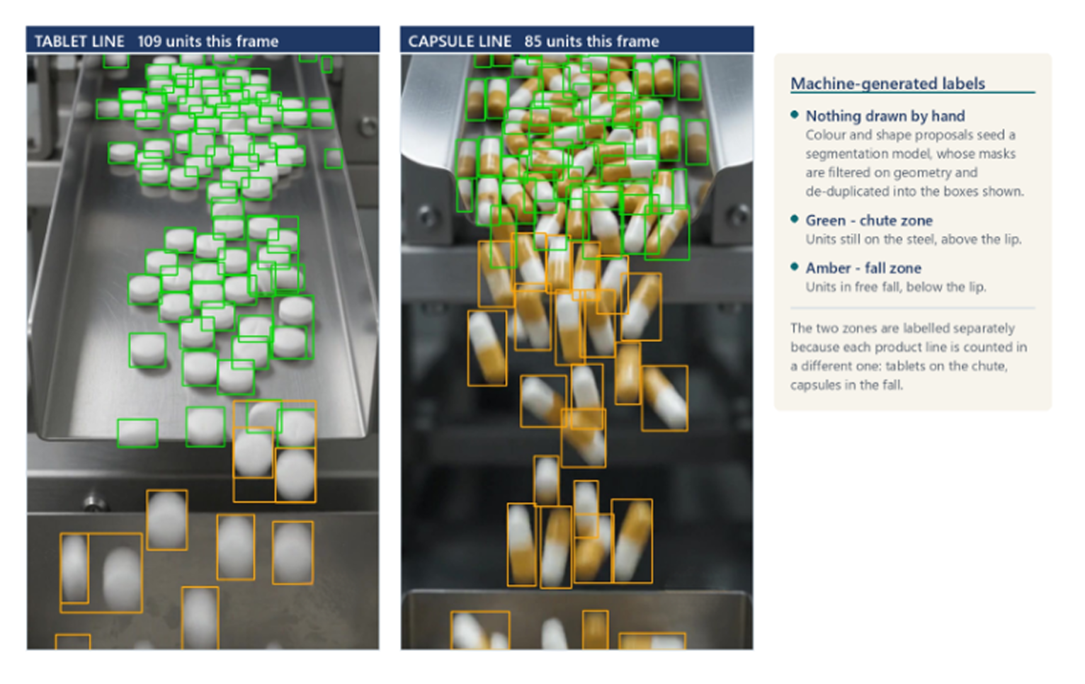
Manual labelling was replaced with an offline pipeline. Candidate regions are proposed by colour and shape analysis, then refined into instance masks by a permissively licensed segmentation foundation model used strictly as a labelling tool. Geometric filters then reject anything whose size, aspect ratio or solidity is inconsistent with a real unit.

Label Quality Control

Nearest-neighbour spacing in object diameters flags duplicates: a cluster closer than physically possible means one object labelled twice. Density anomalies surface missed objects. Where coverage was incomplete, those regions were marked as ignore areas rather than background, so the loss neither rewards nor penalises the model there.

Preprocessing, Training and Export

Frames are letterboxed with symmetric padding so geometry is never distorted, and normalisation is compiled into the exported graph rather than left to application code — removing a category of bug in which training and inference silently disagree about pixel scaling. Training uses a focal objective on the heatmap with masked regions excluded, plus regression losses on the size and offset heads.

Validation

Validation uses two independent mechanisms: The primary one is manual ground truth: a person counts every unit in a held-out test clip and that figure is compared against the system’s count, unit for unit, with each discrepancy inspected to establish its cause. This is laborious, which is why it runs on selected withheld clips rather than continuously — but it is the only method that establishes whether the count is actually right.

The second runs continuously and shares no code with the tracker: an estimator integrates object flux across the counting line, measured density multiplied by measured velocity. It is noisier and is never used as the operational count. Its role is to catch systematic drift — the kind a self-consistent tracker will otherwise report with complete confidence. Results from both appear under Business Impact.

The Algorithm Explained

Detection as Peak-Finding, Not Box-Drawing

The network outputs a low-resolution heatmap: In training every annotated object stamps a small Gaussian at its centre; at inference a local-maximum operation returns object centres directly, while auxiliary maps supply dimensions and a sub-pixel offset.

The advantage is specific: Box detectors must decide, after the fact, whether two overlapping predictions describe one object or two — unanswerable from the boxes alone for identical touching tablets. Peak detection never poses the question. A second benefit: because size is a separate output, both the suppression radius and the tracker’s gates derive from it, so the system adapts to apparent scale without product-specific constants.

Tracking: The Detail That Carried the System

The standard approach initialises each new track at zero velocity and refines its motion model over later observations. Here that fails for a reason no tuning repairs: objects are visible for about five frames while moving fast, so a model beginning at rest never converges before the object has left.

The system therefore divides the frame into horizontal bands, each with a running median velocity. A new track inherits its band’s median, so its first association already knows the object is falling and roughly how fast. The bands are fine enough to capture the acceleration gradient.

Counting, and Where to Place the Line

Its position matters disproportionately. Too high, and units cross before tracks are confirmed; too low, and objects leave view within a frame or two, giving the tracker no chance to correct a mistaken association. The lower-middle of the frame works, and the value stays configurable because it depends on camera geometry.

System Architecture

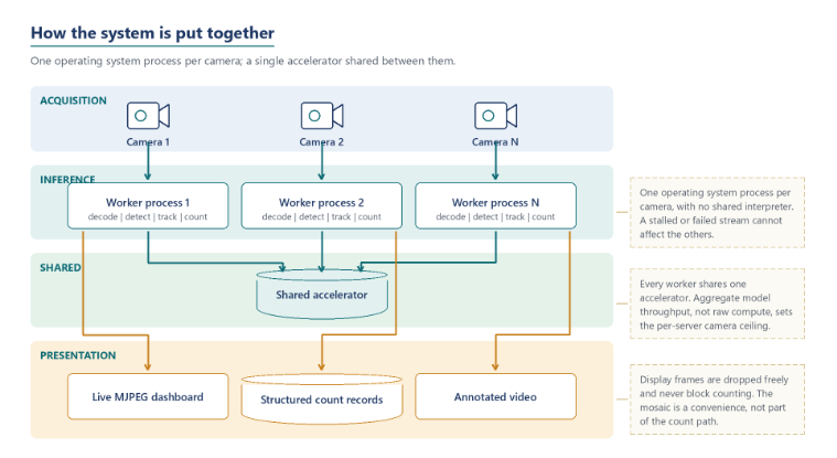
The architecture is deliberately shallow: fewer layers mean fewer failure modes, and in an air-gapped plant every service must be maintained offline.

Acquisition

Camera specification is part of the system, not a procurement detail: a global shutter so fast units are not distorted, exposure of one millisecond or shorter, and at least sixty frames per second so each unit appears in enough frames to be tracked. Diffuse illumination suppresses specular highlights, and the mount must be rigid — the counting line lives in image coordinates, so vibration shifts it relative to the process.

Inference and Aggregation

One process per camera performs decode, preprocessing, inference, suppression, tracking and counting; because the model is small, that chain fits inside a real-time budget on a general-purpose CPU. Processes rather than threads is deliberate: decode, suppression and tracking are interpreter-bound, and separate processes sidestep that contention while sharing one GPU. This was validated, not assumed — an earlier threaded design scaled well on one stream but not across six.

Presentation and Failure Behaviour

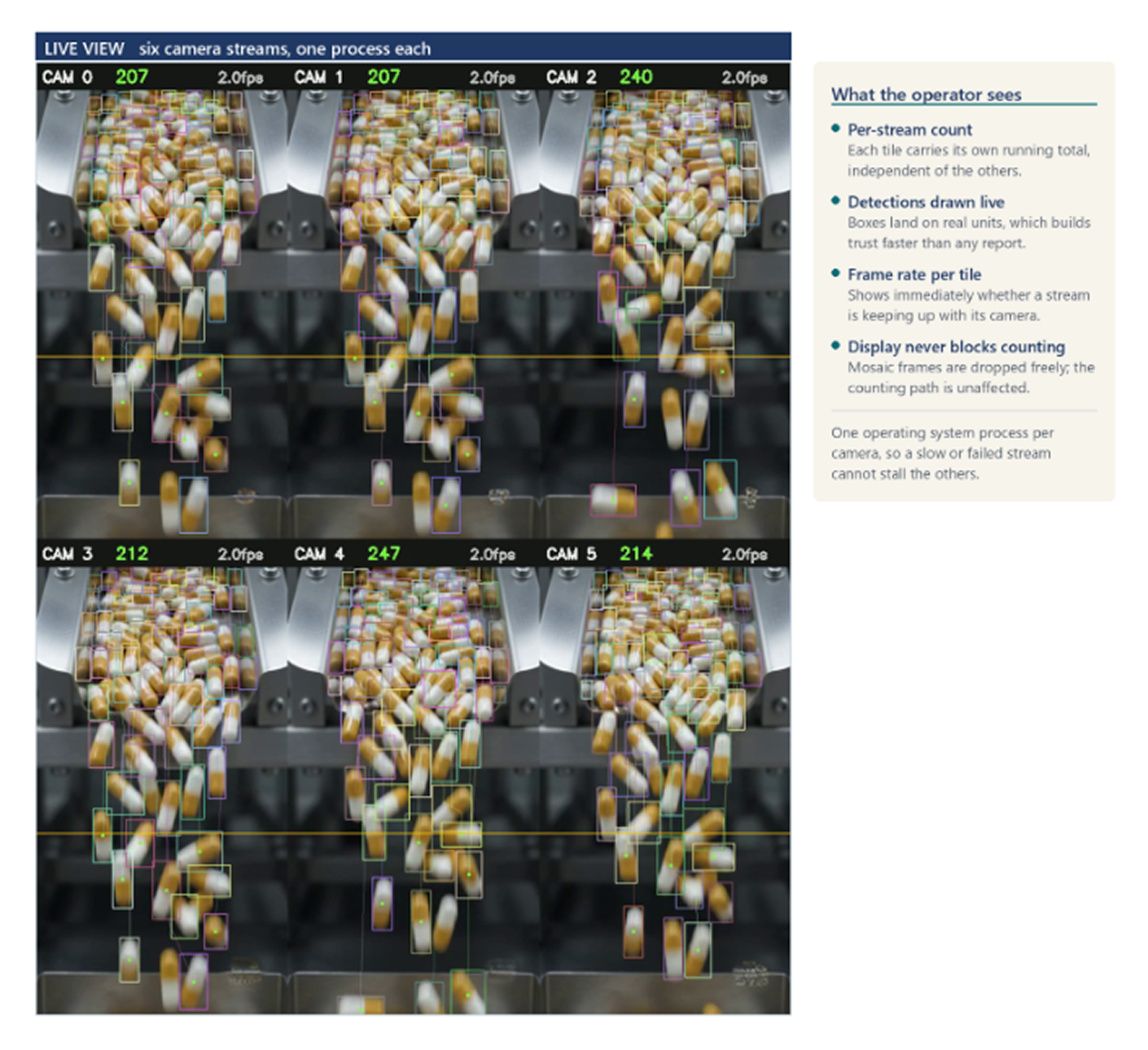
A built-in server streams an annotated live mosaic over standard HTTP, viewable in any browser with nothing to install; display frames are dropped freely, so watching can never slow the system down. Dropped input frames, by contrast, invalidate a run rather than merely slowing it, because they bias the count upward. And when an accelerator is requested but unavailable, the application raises an error rather than quietly using the CPU.

The Intelligent Workflow After AI

The AI-enabled process does not replace existing controls; it inserts a direct measurement where previously there was only inference.

1. Product discharges exactly as before; no mechanical change.
2. A fixed camera observes the discharge region at high frame rate.
3. Units are detected as centre-point peaks, then associated into tracks inheriting their band’s local velocity.
4. Each track crossing the line increments the count once, if supported by a live detection.
5. An independent flux estimator runs in parallel as a continuous sanity check, and counts stream to a live dashboard and a structured record.
6. Checkweigher, reject lane and reconciliation continue unchanged.

The live view also matters on the floor: operators see at a glance that detections land on real units, which does more for trust than any figure in a report.

Before and After

Dimension	Before AI	Before AI
Count measurement	Inferred from total mass; sampled manually	Every unit detected individually at discharge
Coverage	Sample-based in-process checks	Continuous, every unit in view
Detection latency	At checkweigher or batch reconciliation	Real time, at the point of discharge
Sensitivity	Limited by unit-to-unit mass variation	Independent of unit mass entirely
Operator effort	Periodic manual counting	Passive monitoring via live dashboard
Evidence trail	Manual entries and reconciliation	Structured per-stream count and rate records
Line modification	-	None; the camera observes without contact
Connectivity	-	Fully offline; no cloud, no licence server

Business Impact

Deliberately, no financial return figures appear here: return on investment depends on batch economics, deviation rates and labour structures specific to each site, and any number quoted without that context would be invented rather than measured. It is equally worth naming what the system does not do — it does not replace the checkweigher, make a rejection decision or certify a batch. It adds one direct observation where there was none.

Operational Capability Gained

• Direct measurement replaces inference: The count becomes an observed quantity, removing dependence on unit-weight consistency.
• Coverage moves from sample to census: Every unit passing the line is assessed, not a periodic sample.
• Detection shifts left: An anomaly surfaces at discharge rather than at reconciliation, and manual counting becomes passive supervision.
• An objective record is produced: Continuous count and rate data replace manual transcription.

The benefit concentrates where indirect measurement is weakest: small, light units whose absence sits inside the checkweigher’s tolerance, and high-scrutiny products where one deviation dwarfs the monitoring cost. A business case should be built product by product, from the site’s own deviation history.

Measured Counting Accuracy

Counts were verified against manually established ground truth on test clips withheld from training. The table compares two checkpoints of the same tablet detector: one stopped early at 20 epochs, one trained to 320. A third clip was not assessed.

Test clip	Actual	Counted	Missed	False +	Recall
Clip 1 — 20 epochs	438	377	61	0	86.1%
Clip 2 — 20 epochs	355	328	27	0	92.4%
Clip 4 — 20 epochs	343	328	26	11	92.4%
All clips, 20 epochs	1,136	1,033	114	11	89.9%
Clip 1 — 320 epochs	438	432	6	0	98.6%
Clip 2 — 320 epochs	355	352	3	0	99.2%
Clip 4 — 320 epochs	343	355	1	13	99.7%
All clips, 320 epochs	1,136	1,139	10	13	99.1%

Two findings matter more than the headline figure. First, extending training cut missed units elevenfold, from 114 to 10, while precision was unchanged at 98.9 per cent in both runs — the gain came entirely from recall, not from trading one error type for the other. Second, every false positive in both runs occurred on the same clip: eleven from a reflective wall on one side of the conveyor and two from reflections below. Detection error is therefore not randomly distributed but environmental, and it is addressable with baffling or matte surfaces rather than with more training.

The ten residual misses were inspected individually. They fall on frames where the source clip is itself ambiguous — two units merging into a single shape, or a unit briefly vanishing — rather than on cases the model plausibly should have caught. Misses from the early checkpoint had a different and more instructive character: units presenting vertically, units smeared by motion blur, or both. That is the signature of insufficient training rather than of a flawed approach, and it is what the longer schedule resolved.

The capsule detector was reviewed on two clips under the same procedure, missing 42 units on the first and 18 on the second, with losses concentrated where apparent unit size shrinks and where the source footage merges neighbouring capsules. Capsule ground-truth totals are still being finalised, so a recall percentage is deliberately not quoted rather than estimated.

Measured Latency and Throughput

The same production inference code was benchmarked on two machines at opposite ends of the hardware range.

Measurement	Laptop — Core i5-8250U, 4 cores, CPU only	Workstation — Threadripper TRX50 48-core + RTX 4090
Model only, 1 thread	92.8 ms (10.8 fps)	—
Model only, 4 threads / auto	49.6 ms (20.2 fps)	9.4–13.0 ms CPU · 0.97 ms GPU (1,034 fps)
End-to-end, CPU	66.3 ms → 15.1 fps	56–61 fps
End-to-end, GPU	no usable GPU	218 fps
Stage split, best device	decode 3.9 · detect 60.4 · track 2.1 ms	decode 0.80 · detect 3.17 · track 0.62 ms
Against a 24 fps source	0.63× real time	9.1× real time on GPU, 2.4× on CPU

Model-only throughput on the RTX 4090 does not scale monotonically with batch size — it peaks at batch 4 to 8 and then regresses:

Batch size	1	2	4	8	16	32
Throughput (fps)	1,034	1,304	1,497	1,496	1,222	1,101

Accelerated Multi-Stream Pipeline

A second implementation runs the same ONNX model inside NVIDIA DeepStream 7.1, using hardware video decode and a TensorRT FP16 engine, with a custom C++ output parser written for the centre-point heads. The parser was validated offline against the reference NumPy decoder before any GPU was involved: six frames, 444 objects, maximum deviation 0.00000 pixels.

Configuration	Throughput	Objects / frame	Counts per pass
ONNX Runtime + CUDA, 1 stream	218 fps	~75	347 (reference)
DeepStream, 1 stream	807 fps	75.7	—
DeepStream, 6 streams	618 fps aggregate (~103 each)	75.2	—
DeepStream + built-in tracker	—	75.7	202–216
DeepStream + project tracker	—	75.2	339.7 (98% of reference)

Two results are worth drawing out. Detection ported exactly — 75.2 to 75.7 objects per frame against the reference 75 — confirming that the custom parser, the letterbox handling and the FP16 engine are all correct. The counting shortfall was entirely the tracker, and it was structural rather than a tuning problem: counts stayed pinned between 202 and 216 while the built-in tracker’s object yield was pushed from 44.8 to 72.2 per frame across two tracker families and half a dozen configurations. A threshold problem responds to thresholds; this did not. Substituting the project’s own velocity-band tracker recovered 98 per cent of the reference count.

The second result is that aggregate throughput fell from 807 fps on one stream to 618 fps across six, because the counting stage ran single-threaded. That is precisely why the pure-Python deployment path runs one operating system process per camera rather than threads.

Capacity

From the measured stage split, CPU capacity on the 48-core workstation is roughly 13,000 fps aggregate while GPU capacity is 1,034 to 1,497 fps. The GPU therefore binds first, at approximately 17 cameras at 60 fps or 8 at 120 fps. The six-stream figure above is measured; larger camera counts are extrapolated from single-stream numbers and should be confirmed on the target hardware before being committed to.

Technology Stack

Every deployed component was selected for permissive licensing as well as technical fit; the distinction between what is used in development and what ships is maintained rigorously.

Layer	Technology	Role
Acquisition	Industrial global-shutter camera; diffuse illumination	Freeze motion, suppress reflection
Training	PyTorch (BSD-3); rented cloud GPU sessions	Model development only — not deployed
Auto-annotation	Segment Anything (SAM), Apache-2.0	Offline label generation — not deployed
Model format	ONNX with dynamic batch dimension	Portable, framework-independent artefact
Inference runtime	ONNX Runtime (MIT), CPU and CUDA providers	Executes the detector at the edge
Image processing	OpenCV (Apache)	Decode, letterbox, annotation rendering
Application logic	Python; multiprocessing for multi-camera scaling	Tracking, counting, supervision, reporting
Live view	MJPEG over HTTP from the standard library	Browser monitoring, nothing to install
Optional acceleration	NVIDIA DeepStream 7.1 + TensorRT FP16, custom C++ parser	Higher per-stream GPU throughput

Scalability and Future Potential

Scaling Across Lines

The architecture scales by adding worker processes against a shared accelerator. Six concurrent streams at sixty frames per second were sustained on one workstation with no steady-state frame loss and headroom remaining. Sizing follows from accelerator throughput divided by the aggregate frame rate demanded — measured on the intended hardware, not read off headline compute specifications.

Adapting to New Products

A new format requires new training data, and the automated annotation pipeline is what makes that affordable: capture, auto-label, audit, retrain, revalidate. The limitation is worth stating plainly — models trained on one product under one lighting setup do not transfer to a different product on a different conveyor, and predicted sizes do not extrapolate to unseen scales. Onboarding is a data exercise, but not a zero-effort one.

Natural Extensions

Defect and foreign-object detection: The same backbone extends with classes for broken units, colour deviations or foreign material.

Rate analytics and closed-loop control: Density and velocity are already measured, giving early warning of feeder inconsistency; once site validation establishes accuracy, the count can drive rejection directly.

Known Limitations

Camera specification is a hard requirement, not a recommendation: below roughly sixty frames per second, objects do not persist long enough for reliable association. Viewpoint matters — footage from a markedly different angle produced false detections on bare chute surfaces. Reflective side walls within the field of view are the single largest source of false positives measured to date, and are best addressed optically rather than in software. And these models were trained and validated on generated footage; a specific line needs its own capture and retraining cycle before any accuracy claim can be made about it.

Conclusion

Counting objects that move too quickly and sit too closely together to be counted by eye is a problem where the obvious solutions quietly fail. Weight-based inference is blind within its own noise band. Classical image processing drowns in reflections from polished steel. Standard box detection cannot, even in principle, distinguish a duplicate prediction from a genuinely adjacent object. And the most convenient off-the-shelf detectors are ruled out by their licences.

What worked was matching each component to the physics of the problem: centre-point detection rather than box regression, a tracker that starts new objects at the locally observed velocity, automated annotation, and validation by two methods sharing no code. The hard part of an industrial vision system is rarely the model — it is what the camera must be capable of, how labels get produced, how the system behaves when it cannot keep up, and how anyone can tell whether the number it reports is true.

---

Frequently Asked Questions